Solving Mysteries of Exadata Storage Indexes: Part 1

Storage indexes in an Exadata cell server are a somewhat obscure but very important performance benefit for any database — they leverage the available cell server memory to map what range of column values exist in every compression unit (CU) for a table. Once created, they can speed up queries against a table by using this memory-resident “anti-index” to avoid a significant portion of the I/O required for a query even if most of the I/O would occur at the storage level. In earlier Exadata software versions, your tables could have storage indexes created on up to 8 columns; more recent versions of the Exadata cell software can have up to 24 columns indexed.

Storage indexes are somewhat mysterious because you have no direct control over creating them — when a column of a table appears in a join condition or a WHERE clause, a storage index is created after some number of full table scans. Successive queries will use the storage index if the query predicate uses the indexed column. Since I don’t like mysteries, I needed to find out more about how they’re created and used. My investigation was broken down as follows:

1. Create a table with 25M rows and see how to encourage the creation of the storage index and see how fast a storage index is created
2. Use other wait events to see how fast storage indexes are created
3. Validate that up to 24 storage indexes can exist on one table and how they age out of cell server memory
4. Monitor the progress of storage index creation and maintenance
5. Identify inflection points and data distributions that may make storage indexes less useful
6. Latest features of storage indexes in Exadata software
7. Columnar features of storage indexes
8. Contrasting Exadata zone maps and storage indexes

In Part 1, I’ll cover the basics of how storage indexes are automatically created and how to measure the benefits by reductions in physical I/O at the storage layer.

Key Queries

Here are the data dictionary tables and queries I’ll use to measure storage index creation and usage.

The key metric that is exposed by the cell storage environment is statistic #542 that accumulates the number of I/O bytes skipped by using the memory-resident storage index:

select statistic#,name from v$statname 
where name like '%physical%storage%index%';

You can find a full list of the wait events and statistics available in the Oracle Exadata documentation on Monitoring Smart I/O.

I’ll run a query against my test table that has a WHERE clause and will do a full table scan and potentially create a storage index:

SELECT /*+ MONITOR */ MAX(<data_column_name>) 
FROM <test_table>
WHERE <filter_column_expression>;

The query I’ll use at the session level after running searches on the test table will check the total number of bytes saved by the storage index in the session so far:

select statistic#,name,to_char(value,'999,999,999,999,999') value
from v$mystat 
   join v$statname 
      using(statistic#)
where statistic#=542;

Creating the Test Environment

My test table has 26 columns: 25 search columns to use in a WHERE clause, and a “data” column containing the value I was looking for with the search column. This table is based on a similar table that Connor McDonald used to demonstrate the expansion of the number of possible storage indexes from 8 to 24 in this post.

create table t
as select
    trunc(rownum/1000) c1,
    trunc(rownum/1000) c2,
    trunc(rownum/1000) c3,
    trunc(rownum/1000) c4,
. . .
    trunc(rownum/1000) c23,
    trunc(rownum/1000) c24,
    trunc(rownum/1000) c25,
    rpad(rownum,500) data
from
    ( select 1 from dual connect by level < 5001 ),
    ( select 1 from dual connect by level < 5001 );

Because of the Cartesian product of the two “CONNECT BY” queries, I’ll end up with 25 million rows in the table.

Generating and Using Storage Indexes

Once the table is ready, I’ll use an anonymous PL/SQL block to repeatedly query table T on column C1, then immediately check to see if a storage index was created and used.

declare
   scan_count        number;
   maxd              varchar2(500);
   sibytes_prev      number;
   sibytes           number;
begin
   select value into sibytes_prev
   from v$statname s left join v$mystat m 
      on s.statistic#=m.statistic#
   where s.statistic#=542;
   dbms_output.put_line('Session SI bytes saved before running query: ' 
       || to_char(sibytes_prev,'999,999,999,999,999'));
   for scan_count in 1..9
   loop
      execute immediate 
      'select /*+ monitor */ max(data) from t where c1<5000' into maxd;
      select value into sibytes
      from v$statname s left join v$mystat m 
         on s.statistic#=m.statistic#
      where s.statistic#=542;
      dbms_output.put_line('Query exec ' || scan_count || ' I/O bypassed: '
            || to_char(sibytes-sibytes_prev,'999,999,999,999,999'));
      dbms_output.put_line('       SI bytes running total:               '
            || to_char(sibytes,'999,999,999,999,999'));
      sibytes_prev := sibytes;
      -- does storage index need time to be created?
      dbms_session.sleep(5);
   end loop;
end;
/

The loop runs 9 times, and each time calculates the MAX of the “DATA” column. Since it has to do a full table scan to find the MAX value, a storage index on C1 should be created and used; the first time running the SELECT should not use a storage index.

I was pleased to find out that it didn’t take long after the first table scan at the storage level to create a storage index. Subsequent queries using the same column in the predicate returned results more quickly since little or no physical I/O was required to get the results of the query.

Session SI bytes saved before running query:                    0
Query exec 1 I/O bypassed:                    0
       SI bytes running total:                                  0
Query exec 2 I/O bypassed:       14,885,560,320
       SI bytes running total:                     14,885,560,320
Query exec 3 I/O bypassed:       14,885,560,320
       SI bytes running total:                     29,771,120,640
Query exec 4 I/O bypassed:       14,885,560,320
       SI bytes running total:                     44,656,680,960
Query exec 5 I/O bypassed:       14,885,560,320
       SI bytes running total:                     59,542,241,280
Query exec 6 I/O bypassed:       14,885,560,320
       SI bytes running total:                     74,427,801,600
Query exec 7 I/O bypassed:       14,885,560,320
       SI bytes running total:                     89,313,361,920
Query exec 8 I/O bypassed:       14,885,560,320
       SI bytes running total:                    104,198,922,240
Query exec 9 I/O bypassed:       14,885,560,320
       SI bytes running total:                    119,084,482,560

PL/SQL procedure successfully completed.

The SQL Monitoring report for the SELECT statement confirms the observed results. In the I/O section, the “Cell Offload Efficiency” was 86%:

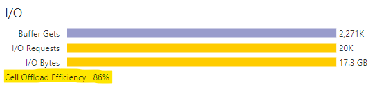
That means 86% of the I/O needed to satisfy the query happened at the storage level and did not have to bring back those rows or columns to the database layer. What about that 14%? Was any of it actual I/O? The details at the last plan line explain the rest:

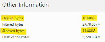
It gets even better — for the table T, which has a total footprint of 25M rows and 18.6 GB in the table segment, the storage index avoided having to do 14.9 GB of those table reads. Out of the remaining eligible bytes, 3.7 GB were read from flash, and after further filtering at the storage layer (remember, offloading can perform row selection and column projection), only 2.7 GB had to be returned to the database layer to calculate the MAX value of the DATA column in the rows where C1 < 5000. In this case, the storage index did the most filtering up front.

Conclusions

You may not have direct control over which columns of which tables will get a storage index created and maintained; however, the conditions which must be present include doing a full table scan of a table in storage using one or more columns of the table as predicates in the WHERE clause. You’re also limited to at most 24 indexed columns in a table — a scenario that seems somewhat unlikely in most applications that have tables in 3rd normal form or even fact tables in a data warehouse database. How fast a storage index will be created on a column and how long it will be maintained are subjects of subsequent posts on this topic.